ECON 4643: Development Economics

Lecture 2: Module 1-Inequality

Author

Harounan Kazianga
Oklahoma State University
Spring 2024

Reading

MB, chap. 10
DR, Chap. 6-8

Motivation

Inequality

Questions of this lecture:
Level of aggregation
Inequality along which dimension?
How to measure inequality?
Why study inequality?

Level of Aggregation

Between countries
Within a country
Among a group of people
Within a household (a family)

Inequality along which dimension?

Income
Should people have access to the same resources? Opportunities?
How should choices and performances be taken into account when considering access to resources?
Consider issues of parental influence
Does inequality serve a purpose or cause incentive to exist?
Should one care about inequality or something else? e.g., social mobility, lifetime wealth?

Why study inequality?

Political and societal aspects
Perception of injustice
Political stability
Pereception of own economic situation relative to others
Is equality something that society should want per se

Measurement of Inequality

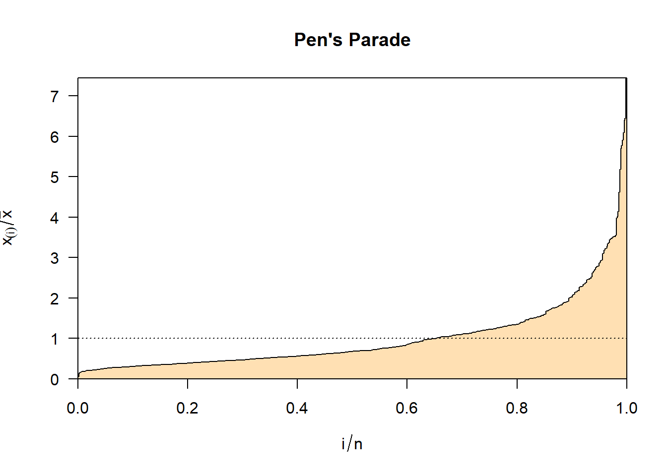
Pen’s parade approach

Graphically depicts how income is distributed across a population, showing the proportion of total income earned by each cumulative percentile of the population.
Extremes are clear
But how to comapare in-between cases?

Pen’s parade approach: Illustration

Principles of Inequality Measures

Economic Inequality

Consider two economies $A=(20,30,50)$ and $B=(22,22,56)$
Easy to say a society such as $(50,50)$ is equal and one such as $(0,100)$ is unequal. What about societies $A$ and $B$ ?
To get an idea of how to compare these two societies we need to agree on some principles that we feel a reasonable measure of inequality should satisfy.
We are going to discuss four principles that get at relative differences in inequality:
Is $A$ more unequal than $B$ ?
Formalization:
Let a society have $n$ people
Income of the $n$ people are $\left\{y_1, y_2, \ldots, y_n\right\}$
Because we are interested in relative inequality we will be comparing $\left\{y_1, y_2, \ldots, y_n\right\}$ and $\left\{y_1^{\prime}, y_2^{\prime}, \ldots, y_n^{\prime}\right\}$

Anonymity Principle

Inequality measure should be independent of who owns the income
Should not mater whether we are looking at a society with $\{100, 200, 300 \}$ or $\{300, 200, 100 \}$
Even if one person feels she would prefer a specific society to the other, can we say one of the above society is more unequal?
This lead to the first principle:
Anonymity Principle: For any distribution of income in a society we can write that distribution as $\left\{y_1, y_2, \ldots, y_n\right\}$ where $y_1 \leq y_2 \leq \ldots \leq y_n$.
For any given society, reordering individuals from the lowest to the highest income does not change inequality in that society.

Population Principle

This principle says that cloning the population should not alter inequality.
If we had a society such as $\{100,200,300\}$ and cloned each individual so that we had society $\{100,100,200,200,300,300\}$ should we consider one of these societies more or less equal than the other?
This means that all that matters are the proportions of the population that earn different levels of income.
This leads us to our second principle:
Population Principle: If we compare an income distribution over $n$ people and another population of $2 n$ people with the same income pattern repeated twice, there should be no difference in inequality between the two income distributions.

Relative Income Principle

Consider distributions $\{100,200,300\}$ and $\{200,400,600\}$. Should we say that one economy is more unequal than the other?
In terms of development the level of income might matter (such as in the level of per capita income) but not in terms of inequality.
Inequality represents how people’s income are in relative terms. Therefore a measure of inequality should not be subject to the absolute level of incomes.
Thus the third principle:
Relative Income Principle: It is tantamount to the assertion that income levels, in and of themselves, have no meaning as far as inequality measurement is concerned. Thus the inequality in $\{100,200,300\}$ is equal to the inequality in $\{200,400,600\}$.

Dalton Principle

If we take money from someone who is poorer and give it to someone richer in a society what should we say about inequality in that society?
Example: compare $Y_1 = \{90,200,310\}$ to $Y_2 = \{100,200,300\}$ Which is more unequal?
We formalize this idea below:
Dalton Principle: Consider $\left\{y_1, y_2, \ldots, y_n\right\}$ such that $y_1 \leq y_2 \leq \ldots \leq y_n$ and consider incomes $y_i$ and $y_j$ such that $y_i \leq y_j$. A transfer of money from $y_i$ to $y_j$ will be called a regressive transfer. If one income distribution $Y_1$ can be obtained from another income distribution $Y_2$ through a regressive transfer then $Y_1$ has a higher level of inequality.
- In the above example, we can obtain $Y_1$ by applying using a regressive transfer on $Y_2$, i.e. transferring $\$10$ from the poorest individual to the richest individual. Therefore, $Y_1$ is more unequal than $Y_2$.

Lorenz Curves

We will look at these 4 principles apply to Lorenz Curves
Consider an income distribution and calculate the following:
- Percentage Share of total income earned by the bottom $x \%$ of the population. Where $x \in[0,100 \%]$
If we plot this percentage share on the $x$-axis with the amount of income that share has on the $y$-axis we will get the Lorenz Curve of that income distribution.
Note: Perfect equality $\Rightarrow 45^{\circ}$-line is the Lorenz Curve.
Note: As our Lorenz curve moves further away from the $45^{\circ}$-line inequality $\Uparrow$

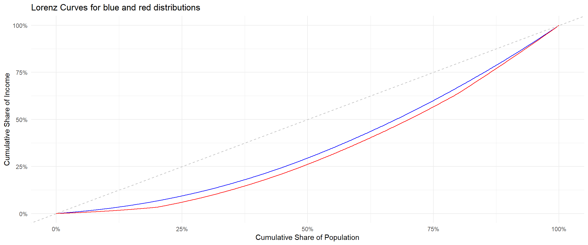
Lorenz curves: Easily Comparable Case

Lorenz Curves

Lets now compare to income distributions $Y=\left\{y_1, y_2, \ldots, y_n\right\}$ and $Y^{\prime}=\left\{y_1^{\prime}, y_2^{\prime}, \ldots, y_n^{\prime}\right\}$
Say that the Lorenz curve associated with income distribution $Y$ is $L_Y$ and the Lorenz curve associated with income distribution $Y^{\prime}$ is $L_{Y^{\prime}}$.
We say an income distribution $Y^{\prime}$ is more unequal compared to $Y$ if $L_{Y^{\prime}} \leq L_Y$ for all $x \% \in[0,100 \%]$.
We can see this easier if we graph both curves and will do so shortly.
Note that if $L_{Y^{\prime}}$ is below $(\leq) L_Y$ for all values of $x \%$ then the poorer people in $L_Y$, have less of a share of the income when compared to the same $x \%$ of the population in $L_Y$.
We say an inequality measure is Lorenz-Consistent for $Y$ and $Y^{\prime}$ it is true that $L_{Y^{\prime}} \leq L_Y$ for all $x \% \in[0,100 \%]$.
Theorem: An inequality measure is Lorenz-Consistent if and only if it is simultaneously consistent with the anonymity, population, relative income and Dalton principles.

Lets look at how the Dalton Principle is satisfied with the Lorenz criteria.
If money is taken from someone who has income $y_j \leq y_i$ then the cumulative income held by the people $1,2, \ldots, i$ is less then before and the cumulative income held by the people $j, j+1, \ldots, n-1, n$ is more.
Therefore the Lorenz curve after this regressive transfer should move further away from the $45^{\circ}$-line.
In the previous figure:
- The distribution in blue is more equal than the one in red
- The distribution in red is obtained from the one in blue by transferring income from the bottom 20% to the top 80% of the income distribution, i.e. by applying a regressive transfer
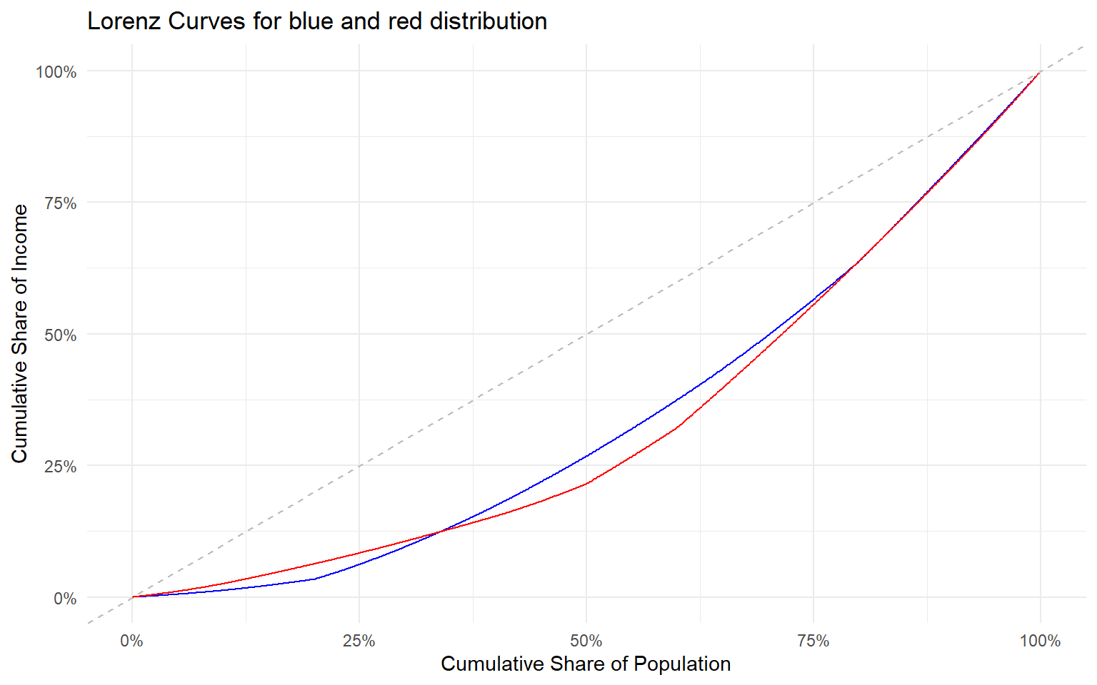
Unfortunately, though, the Lorenz curve can lead to lots of cases where we cannot compare inequality within two countries.
If two Lorenz curves cross $\Rightarrow$ No clear comparison can be made regarding inequality.
If there exists some $x \%$ such that $L_1(x)>L_2(x)$ and there exists some $y \%$ such that $L_1(y)<L_2(y)$ then we say that the Lorenz curves for income distributions 1 and 2 cross.
In this case we cannot go through a series of transfers from one economy to the next, using our set of principles, to arrive at a conclusion of which income distribution is more unequal.
Consider the following graph.

Lorenz Curves: Inconclusive Case

The Gini Coefficient

When Lorenz curves bring ambiguous results many people turn to the Gini coefficient.
The Gini coefficient is a complete ranking - it spits out a number for every conceivable distribution.
Besides the Gini coefficient there are other complete rankings we can look at; such as the range, Kuznets ratios, mean absolute deviation, and coefficient of variation.
We need more formality before discussing these other measures, though. Say:
There are $m$ distinct incomes
- $n_j$ people are earning income in class $j$
- $n$ is the total number of people and is $n=\sum_{j=1}^m n_j$
- $\mu$ is the mean of a distribution and is defined $\mu=\frac{1}{n} \sum_{j=1}^m n_j y_j$

The Gini Coefficient

-We can now define the Gini-coefficient:

\[ G=\frac{1}{2 n^2 \mu} \sum_{i=1}^m \sum_{j=1}^m n_i n_j\left|y_i-y_j\right| \]

The Gini is actually defined on the sum of all pair-wise comparisons of income in the population.
The Gini-coefficient satisfies all four of the properties we checked earlier.
There is also a graphical interpretation that may help you to remember the Gini-coefficient:
It is the ratio of the area between the Lorenz curve and the $45^{\circ}$-line and the area under the $45^{\circ}$-line as a whole.

The Gini Coefficient

Gini-Coefficient can be thought of as $G=\frac{A}{A+B}$ where $A$ and $B$ are as illustrated below.

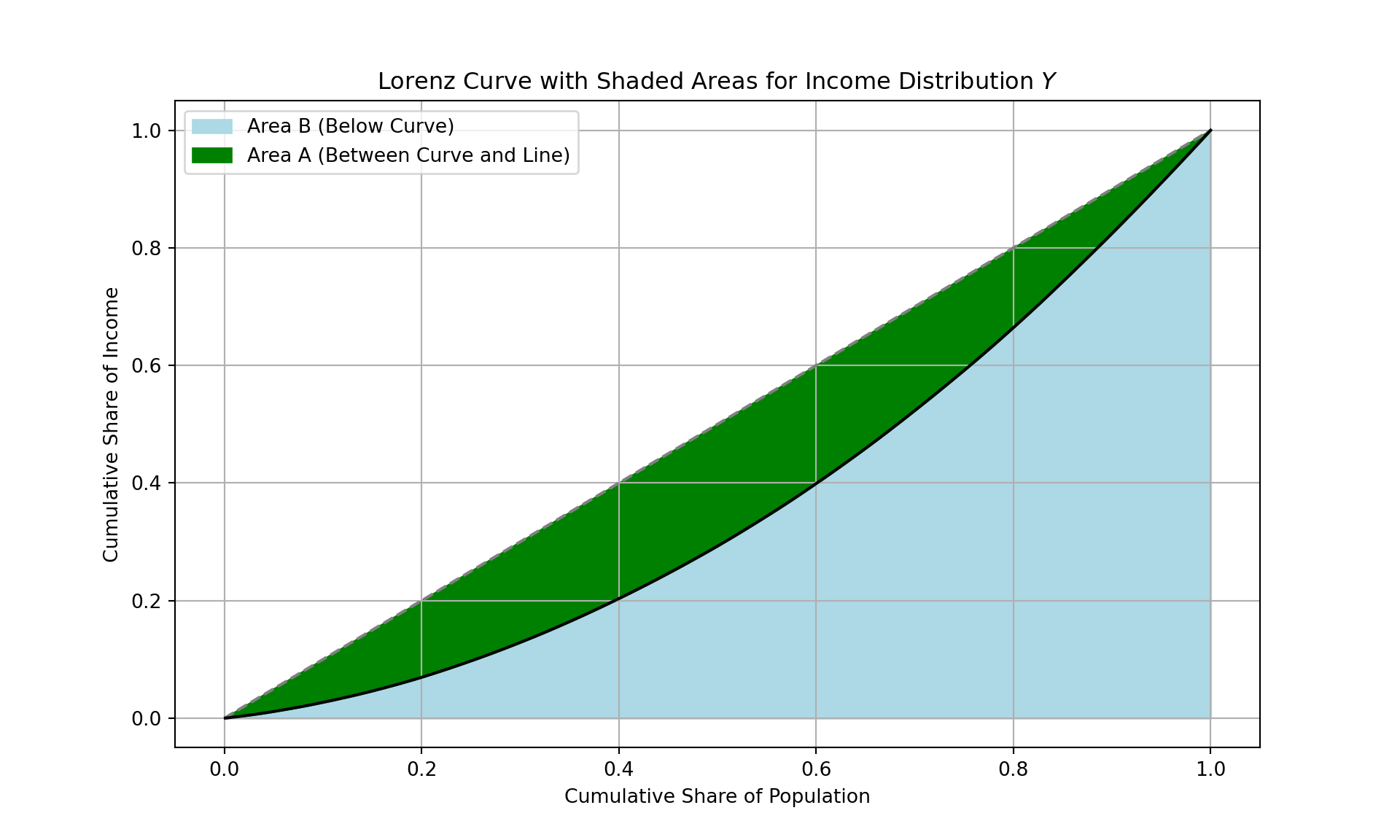
Illustration

Graph the Lorenz curve, using 10 observations

Code

# Load ggplot2 library
library(ggplot2)

# Income data
income <- c(9, 18, 10, 10, 19, 3, 2, 5, 11, 17)

# Sort the income data in ascending order
income <- sort(income)

# Calculate the cumulative share of income
cum_income <- cumsum(income) / sum(income)

# Calculate the cumulative share of the population
pop <- 1:length(income) / length(income)

# Create a data frame for plotting
df <- data.frame(pop, cum_income)

# Plot the Lorenz Curve using ggplot2
ggplot(df, aes(x = pop, y = cum_income)) +
  geom_line(color = "blue") +
  geom_abline(slope = 1, intercept = 0, color = "red", linetype = "dashed") +
  xlab("Cumulative Share of Population") +
  ylab("Cumulative Share of Income") +
  ggtitle("Lorenz Curve") +
  theme_minimal()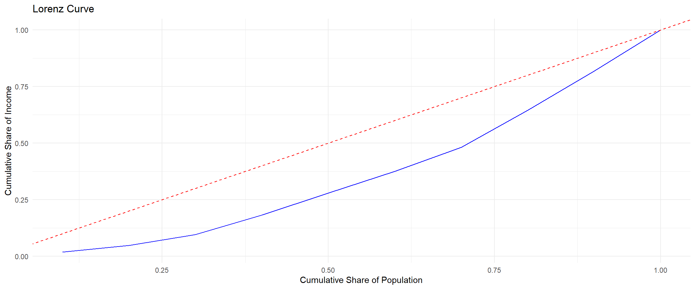

Illustration

Gini Coefficient, using 10 observations.
- We apply $G=\frac{1}{2 n^2 \mu} \sum_{i=1}^m \sum_{j=1}^m n_i n_j\left|y_i-y_j\right|$

Code

# Income data
income <- c(9, 18, 10, 10, 19, 3, 2, 5, 11, 17)

# Calculate mean income (mu)
mu <- mean(income)

# Number of entities (n)
n <- length(income)

# Initialize sum of absolute differences
sum_abs_diff <- 0

# Compute the double summation of absolute income differences
for (i in 1:n) {
  for (j in 1:n) {
    sum_abs_diff <- sum_abs_diff + abs(income[i] - income[j])
  }
}

# Calculate the Gini coefficient
gini_coefficient <- (1 / (2 * n^2 * mu)) * sum_abs_diff

# Print the Gini coefficient
print(gini_coefficient)

[1] 0.3115385

Other complete measures of inequality

The Range: \[ R=\frac{1}{\mu}\left(y_m-y_1\right) \]
Kuznets ratios: ratio of the shares of income of the richest $x \%$ to the poorest $y \%$ where $x$ and $y$ stand for numbers such as 10,20 , or 40. Example given, the $\frac{20}{40}$-ratio.
Mean Absolute Deviation: \[ M=\frac{1}{\mu n} \sum_{i=j}^m n_j\left|y_i-\mu\right| \]
Coefficient of variation: \[ C=\frac{1}{\mu} \sqrt{\sum_{j=1}^m \frac{n_j}{n}\left(y_j-\mu\right)^2} \]

Why Study Inequality

If we do not care about inequality itself we may care about how it affects income or growth.
Savings rates are effected by income levels.
Inequality could provide incentives for people to work harder to reach a different social status.
Access to credit and finance is constrained.
We must focus on the causal story, i.e. does inequality cause…?
We will look at the Kuznet’s curve and then four potential models of why income inequality and growth may be related.

Inequality and Development: The Kuznets Hypothesis

Kuznets hypothesized that there was an inverted-U shaped relationship between inequality and development.
Kuznets suggested that: economic progress, measured by per capita income, is initially accompanied by rising inequality, but these disparities ultimately go away as the benefits of development permeate more widely. -Low-level of income $\Rightarrow$ Low inequality.
- Moderate-levels of income $\Rightarrow$ High inequality.
- High-levels of income $\Rightarrow$ Low inequality.
Two ways to test this relationship:
Look at countries over a long period of time: Time Series.
Look at a group of countries at one point in time: Cross-Section.
We will use a cross-sectional approach.

Inequality and Development: The Kuznets Hypothesis

How to test Kuznets’ hypothesis?
Let $s_i$ be the share of total income going to group $i$.
Let $y$ be the level of per capita income.
As $y \Uparrow$ we expect that the share of income held by the richest $20 \%$, $s_{20}$ will at first $\Uparrow$ and then $\Downarrow$.
As $y \Uparrow$ we expect that the share of income held by the poorest $20 \%$ $s_p$ will at first $\Downarrow$ and then $\Uparrow$.
To test this relationship we can use the following regression: \[ s_i=A+b y+c y^2+D+\varepsilon \]
What signs should each of the coefficients take?
Ahluwalia analyzed a sample of sixty countries: 40 developing; 14 developed; 6 socialist.
Ahluwalia used the above equation to test the Kuznets inverted-U hypothesis… What do you think he found?

Inequality and Development: The Kuznets Hypothesis

Ahluwalia' results
Income Share	$y $	$y^2$	Socialist Dummy	$R^2$
Top 20%	89.85 (4.48)	17.56 (4.88)	-20.15 (6.83)	0.58
Middle 40%	-45.59 (3.43)	9.25 (3.88)	8.21 (4.20)	0.47
Lowest 20%	-16.97 (3.71)	3.06 (3.74)	5.54 (8.28)	0.54

Ahluwalia found that the Kuznets hypothesis holds.
What do you think about these results?
What else could be done to test the inverted-U hypothesis?
Do you believe Ahluwalia’s results?
There are many data examples in the book BUT the general message is that the Kuznets’ inverted-U hypothesis probably does not hold except in a small number of cases.