Code
if (!require("pacman")) install.packages("pacman")Loading required package: pacmanCode
pacman::p_load(haven, DescTools, knitr, kableExtra, ineq, ggplot2, formatdown, tidyverse, WDI)Lecture 4: Module 1-Growth
if (!require("pacman")) install.packages("pacman")Loading required package: pacmanpacman::p_load(haven, DescTools, knitr, kableExtra, ineq, ggplot2, formatdown, tidyverse, WDI)ED Ch 3
At the macro level, successful development requires a combination of:
Reduction in inequality
Reduction poverty and vulnerability
Economic growth
We now turn to economic growth (after having discussed inequality and poverty in Lectures 2 and 3)
Economic growth is:
The rate of increase in a country’s average income.
Total income equals the total value of production, so the rate of economic growth rate is positive when aggregate labor productivity is rising.
Economic growth is usually measured as the average annual rate of growth in real per capita gross domestic product (GDP).
Economic growth is necessary for development
But economic growth is not sufficient for full development success
Reading Assignment (on Canvas): Easterly, W (2001) ``The Political Economy of Growth Without Development: A Case Study of Pakistan’’
Four-minute video in which statistician Hans Rosling provides a visual history of growth and development around the world over the last 200 years: http://www.flixxy.com/200-countries-200-years-4-minutes.htm
Proximate Sources: The kinds of change in socioeconomic activity that give rise to economic growth and the related choices through which those changes come about.
Economic determinants: The types of policies, institutions, external market conditions, and other circumstances that are taken as given by people within the socioeconomic system, and that affect how willing and able people are to make the choices associated with the proximate sources of growth
Political determinants: The political conditions that lead policymakers to put good policies and institutions into place
Economic growth involves growth in aggregate labor productivity.
Economists begin their study of productivity by thinking about the many firms throughout the economy in which production takes place.
Economists organize their thinking about the technological possibilities a firm faces around the concept of a production function.
\[ Y = F\left(L, K; A\right) \]
Where \(Y\) is output quantity \(L\) is labor \(K\) is capital \(A\) represents total factor productivity
We will make frequent reference to the following - the average product of labor \[AP_L = \frac{Y}{L} = \frac{F\left(L, K; A\right)}{L} \]
\[AP_K = \frac{Y}{K} = \frac{F\left(L, K; A\right)}{K} \]
- the marginal product of labor \[
MP_L = \frac{\partial F\left(L, K; A\right) }{\partial L}
\] or \(\frac{\Delta Y}{\Delta L}\)
the marginal product of capital \[ MP_L = \frac{\partial F\left(L, K; A\right) }{\partial K} \] or \(\frac{\Delta Y}{\Delta K}\)
We expect:
Illustration: suppose that the production function is
\[ Y=4 L K+0.1 L^2 K+0.2 L K^2-0.04 L^3 K-0.02 L K^3 \] In this case, the average product of labor is
\[ \text{APL} = \frac{Y}{L} = 4K + 0.1LK + 0.2LK^2 - 0.04L^2K -0.02K^3 \] and the marginal product of labor is
\[ \text{MPL} = \frac{\partial Y}{\partial L} = 4K + 0.2LK + 0.2K^2 - 0.12LL^2K - 0.02K^3 \] The R-chunk below will take a value of capital \(K\), the maximum size of labor \(n\) and a technology shifter \(A\), and then generate a table of output (Table 1), and average and marginal products.
production_data <- production_function(K = 3, n = 15, A=5)
#print(production_data)

kable(production_data)| Labor | Capital | Output | APL | MPL |
|---|---|---|---|---|
| 0 | 3 | 0.00 | NA | 1.26 |
| 1 | 3 | 16.44 | 16.44 | 6.50 |
| 2 | 3 | 32.76 | 16.38 | 11.02 |
| 3 | 3 | 48.24 | 16.08 | 14.82 |
| 4 | 3 | 62.16 | 15.54 | 17.90 |
| 5 | 3 | 73.80 | 14.76 | 20.26 |
| 6 | 3 | 82.44 | 13.74 | 21.90 |
| 7 | 3 | 87.36 | 12.48 | 22.82 |
| 8 | 3 | 87.84 | 10.98 | 23.02 |
| 9 | 3 | 83.16 | 9.24 | 22.50 |
| 10 | 3 | 72.60 | 7.26 | 21.26 |
| 11 | 3 | 55.44 | 5.04 | 19.30 |
| 12 | 3 | 30.96 | 2.58 | 16.62 |
| 13 | 3 | -1.56 | -0.12 | 13.22 |
| 14 | 3 | -42.84 | -3.06 | 9.10 |
| 15 | 3 | -93.60 | -6.24 | 4.26 |
# Plot APL and MPL against Labor using ggplot2
ggplot(production_data, aes(x = Labor)) +
  geom_line(aes(y = APL, colour = "APL"), size = 1) + # Plot APL
  geom_line(aes(y = MPL, colour = "MPL"), size = 1) + # Plot MPL
  labs(title = "APL and MPL against Labor",
       x = "Labor",
       y = "Productivity",
       colour = "Measure") +
  scale_colour_manual(values = c("APL" = "blue", "MPL" = "red")) +
  theme_minimal()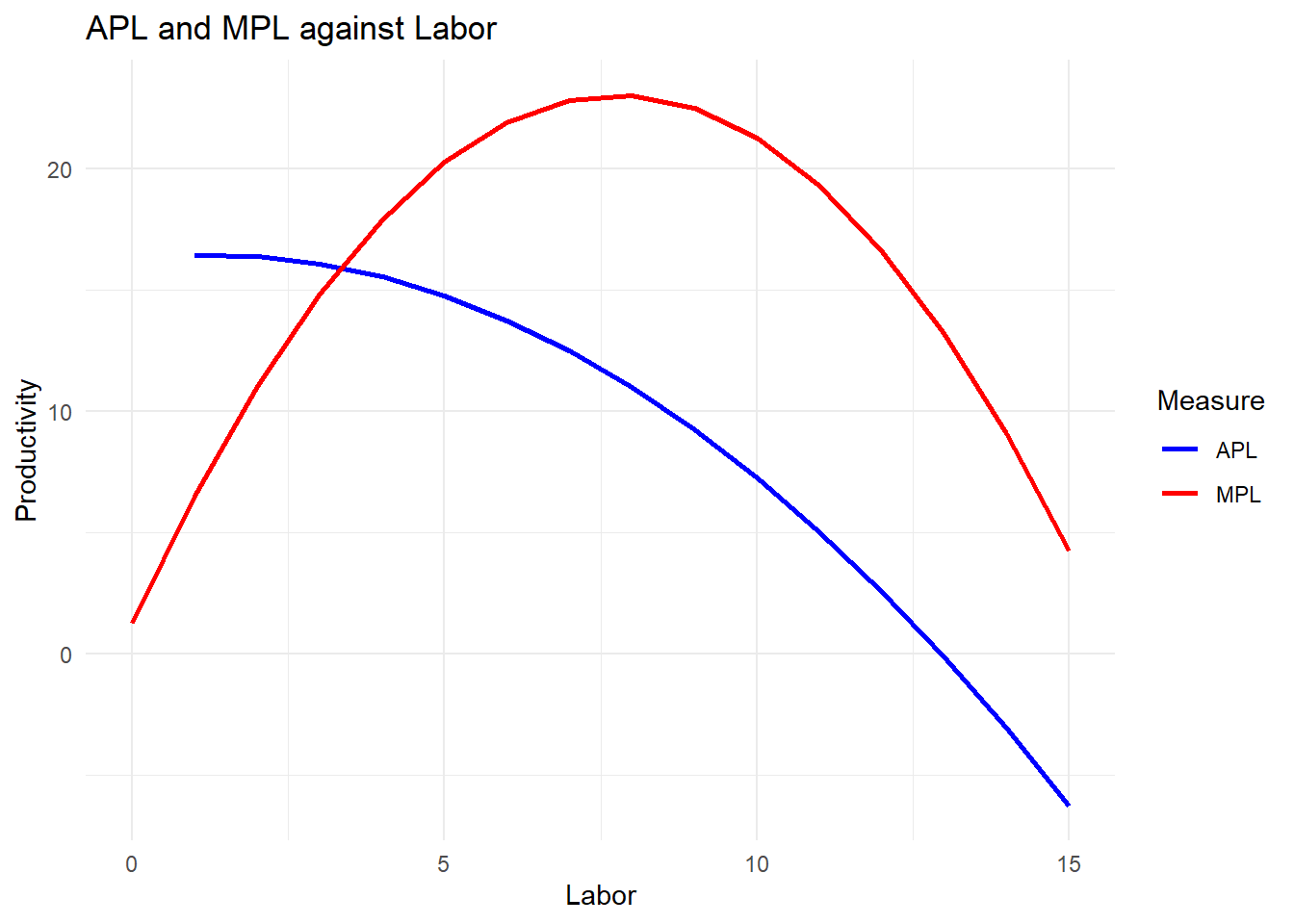
Now, we can explore what happens if we increase capital from \(K=3\) to \(K=6\).
production_data_K6 <- production_function(K = 6, n = 15, A=5)

# Plot APL and MPL against Labor for both K = 10 and K = 15 using ggplot2
ggplot() +
  geom_line(data = production_data, aes(x = Labor, y = APL, colour = "APL K=3"), size = 1) +
  geom_line(data = production_data, aes(x = Labor, y = MPL, colour = "MPL K=3"), size = 1) +
  geom_line(data = production_data_K6, aes(x = Labor, y = APL, colour = "APL K=6"), size = 1, linetype = "dashed") +
  geom_line(data = production_data_K6, aes(x = Labor, y = MPL, colour = "MPL K=6"), size = 1, linetype = "dashed") +
  labs(title = "APL and MPL against Labor for K=3 and K=6",
       x = "Labor",
       y = "Productivity",
       colour = "Measure") +
  scale_colour_manual(values = c("APL K=3" = "blue", "MPL K=3" = "red", "APL K=6" = "darkblue", "MPL K=6" = "darkred")) +
  theme_minimal()
The discussion of firms suggests that at the aggregate level, average labor productivity can grow through:
Accumulation of physical capital (more rapid than the rate of growth of population)
Accumulation of human capital (increasing average skill level of workforce)
Improvements in technology (through research, development, dissemination, purchase and adoption of new technologies)
Improvements in technical efficiency
At the aggregate level, average labor productivity may also grow through re-allocations of labor across activities that:
Shift labor from sectors or firms where the value of the marginal product of labor (VMPL) is lower to sectors or firms where the VMPL is higher
Shift labor out of unemployment into employment
Shift labor out of rent-seeking activities into productive activities
Accumulation of assets
Physical capital
Human capital
Improvements of technology
Improved efficiency in utilsation of assets
Growth accounting studies seek to quantify the relative importance of factor accumulation (i.e. rising quantities of physical or human capital per worker) and growth in total factor productivity (i.e. all other proximate sources of growth) for explaining historical growth.
Often they find that factor accumulation and TFP growth each explain about half of overall growth.
Development accounting studies seek to quantify the relative importance of differences in physical or human capital per worker and differences in TFP for explaining differences across countries in GDP per worker.
Often they find that differences in capital per worker and differences in TFP each explain about half of the cross-country differences.
Empirical observations suggest that developing countries have room to improve in all of these areas.
Why do capital accumulation, technical change, improvements in efficiency and reductions in waste happen more rapidly in some countries than others?
Determinants considered in cross-country growth regression literature:
\[ \frac{\Delta w}{w} + \frac{\Delta z} {z} \]
\[ \frac{\Delta w}{w} - \frac{\Delta z} {z} \]
\[ G = \left( \frac{y_T}{y_0} \right)^{\frac{1}{T}} - 1 \] -This is easily calculated with a handheld calculator.
\[ g = \frac{ln y(t) - ln y(0)}{t} \]
\[ G \simeq \frac{ln\frac{y_t}{y_0}}{t} = g \]
If given the growth rate, we can estimate how long it would take for the vatiable to double (or triple, etc.)
With discrete time, we know that: \[ 1 + G=\left(\frac{y_T}{y_0}\right)^{\frac{1}{T}} \]
Take the natural log of both sides and solve for \(T\)
GDP doubling means that \(\frac{y_T}{y_0} = 2\), so we can substitute to get
\[ T = \frac{ln(2)}{ln (1 + G)} \simeq \frac{0.6931}{ln(1+ G)} \]
The basic growth model is based on five equations:
Aggregate production function \(Y = F(K, L)\)
Saving \(S\) depends on income \(Y\), and \(s\), i.e. \(S=s Y\). Example: if \(s=.20\) and \(Y=10\) billions, then saving is \(S=2 B\)
Investment \(I\) is funded with saving; \(\mathrm{S}=\mathrm{I}\) (Saving=Investment)
Change in \(\Delta \mathrm{K}=(\mathrm{I}-\mathrm{dK})\) where \(\mathrm{d}=\) depreciation and \(\mathrm{K}=\) capital
Change in \(\Delta \mathrm{L}=\mathrm{nxL} \mathrm{n}=\) population growth and \(\mathrm{L}=\mathrm{Labor}\) force, If \(\mathrm{L}=1\) mill. & \(\mathrm{n}=.02\)
Combining 2,3,4, leads to \(\Delta \mathrm{K}=\mathrm{sY}-\mathrm{dK}\)
5 equations and 5 variables can be solved and the change in \(\mathrm{K}\) can be substituted into Production function \(\mathrm{Y}=\mathrm{f}(\mathrm{K}, \mathrm{L})\)
The HD Growth model is a particular model with basic feature of fixed coefficient production function.
It assumes no substitution between labor and capital \(\mathrm{Q}= F\left( K, L \right) = \min \mathrm{F}(\mathrm{L}, \mathrm{K})\) : the production Isoquant is L shaped
It also shows constant returns to scale (CRS) i.e. doubling inputs will double output as you can see in Figure 3
# Adjust the Leontief production function to Y = min(K, L)
hdpf <- function(K, L) {
  pmin(K, L)
}

# Generate a grid of K and L values
K_range <- seq(0, 50, length.out = 100)
L_range <- seq(0, 50, length.out = 100)

# Create a dataframe for plotting
grid <- expand.grid(K = K_range, L = L_range)
grid$Y <- with(grid, hdpf(K, L))

# Isoquant levels for specific combinations
Y1 <- hdpf(10, 20)
Y2 <- hdpf(20, 40)

# Base plot
p <- ggplot(grid, aes(x = K, y = L)) +
  geom_contour(aes(z = Y, colour = factor(stat(level))), breaks = c(Y1, Y2)) +
  scale_colour_manual(values = c('blue', 'red'),
                      name = "Isoquant",
                      labels = c("Isoquant I (K=10, L=20)", "Isoquant II (K=20, L=40)")) +
  labs(title = "HD Production Function Isoquants: Y = min(K, L)",
       x = "Capital (K)", y = "Labor (L)") +
  theme_minimal() +
  coord_fixed(ratio = 1)  # Ensure the same scale for both axes

# Print the plot
print(p)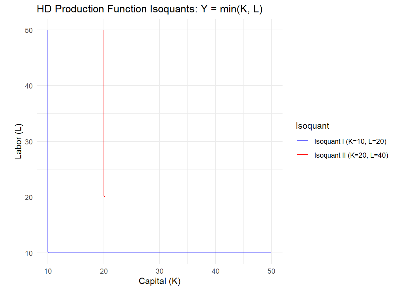
Let \(Y\) (income) be GDP and \(S\) be savings. The level of savings is a function of the level of GDP as before, say \(S = sY\).
The level of capital \(K\) needed to produce an output \(Y\) is given by the equation \(K = vY\), where \(v\) is the incremental capital-output ratio (ICOR), and \(v = \frac{K}{Y}\)
From \(K = vY\), we get \(\Delta K = v \Delta Y\)
From equation 4 above, \(\Delta \mathrm{K}=\mathrm{I}-\mathrm{dK}\)
Combining (a) and (b), we get:
Notice that the left hanside term of the last equation is just the growth rate of \(Y\) (GDP). Thus, in the basic HD model, the growth rate is \(Y_g = \left(\frac{s}{v}\right) - d\)
The policy prescription of the model is straightforward: promote saving to accelerate growth.
Suppose that the propensity to consume is \(c = 0.76\). The capital (\(K\)) stock is \(3,000\) units, GDP (\(Y\)) is \(1,000\), and the depreciation rate (\(d\)) is \(0.05\). What is the growth rate of this economy?
countries <- c("KE", "MX", "CN", "CI", "VN") # ISO2 country codes
indicators <- c(GFCF = "NE.GDI.FTOT.ZS", GDP_Growth = "NY.GDP.MKTP.KD.ZG")

# Fetch data for 2010 and 2019
wdi_data <- WDI(indicator = indicators, country = countries, start = 2010, end = 2019, extra = FALSE)
# Calculating averages for each indicator across 2015 to 2020 for each country
avg_data <- wdi_data %>%
  group_by(country) %>%
  summarize(GFCF_Percent_GDP =  mean(GFCF, na.rm = TRUE),
            GDP_Annual_Growth_Percent = mean(GDP_Growth, na.rm = TRUE)) %>%
  mutate(ICOR = GFCF_Percent_GDP/GDP_Annual_Growth_Percent)

knitr::kable(avg_data,
      format = "html",
      col.names=c("Country", "Gross fixed capital formation (% of GDP)", "GDP growth (annual %)", "ICOR"),
      digits = 2,
      full_width = F, position = "float_top",
      format.args = list(big.mark = "," , scientific = FALSE))%>%
footnote(c("Source: World Bank, World Development Indicators", "Adapted from de Janvry and Sadoulet (2021), Table 8.1"))| Country | Gross fixed capital formation (% of GDP) | GDP growth (annual %) | ICOR |
|---|---|---|---|
| China | 43.16 | 7.68 | 5.62 |
| Cote d'Ivoire | 21.13 | 6.24 | 3.39 |
| Kenya | 20.72 | 5.03 | 4.12 |
| Mexico | 22.82 | 2.34 | 9.77 |
| Viet Nam | 30.24 | 6.58 | 4.60 |
| Note: | |||
| Source: World Bank, World Development Indicators | |||
| Adapted from de Janvry and Sadoulet (2021), Table 8.1 |
Builds on the Harrod–Domar model
Adds several neoclassical features
Incorporates total factor productivity (TFP)
Maintains constant returns to scale assumption (Harrod–Domar)
Figure 4 show the isoquants of a Cobb-Douglas production function, with \(A=1\), and \(\alpha=1\)
# Define the Cobb-Douglas production function
cobb_douglas_production <- function(K, L) {
  K^0.5 * L^0.5
}

# Target output levels
Y_targets <- c(10, 20)

# Generate a grid of K and L values
K_range <- seq(1, 50, length.out = 100)  # Start from 1 to avoid division by zero
L_range <- seq(1, 50, length.out = 100)

# Create a dataframe for plotting isoquants
isoquants <- data.frame(K = numeric(), L = numeric(), Output = numeric(), Isoquant = factor())

# Calculate K and L combinations for each Y target
for (Y in Y_targets) {
  for (K in K_range) {
    L <- (Y / (K^0.5))^2
    if (L <= 50) {  # Include only the combinations within the specified L range
      isoquants <- rbind(isoquants, data.frame(K = K, L = L, Output = Y, Isoquant = as.factor(Y)))
    }
  }
}

# Plot the isoquants
ggplot(isoquants, aes(x = K, y = L, colour = Isoquant)) +
  geom_line() +
  scale_colour_manual(values = c("10" = "red", "20" = "blue"),
                      name = "Output Level",
                      labels = c("Y = 10", "Y = 20")) +
  labs(title = "Cobb-Douglas Production Function Isoquants",
       x = "Capital (K)", y = "Labor (L)") +
  theme_minimal() +
  coord_fixed(ratio = 1)  # Ensure the same scale for both axes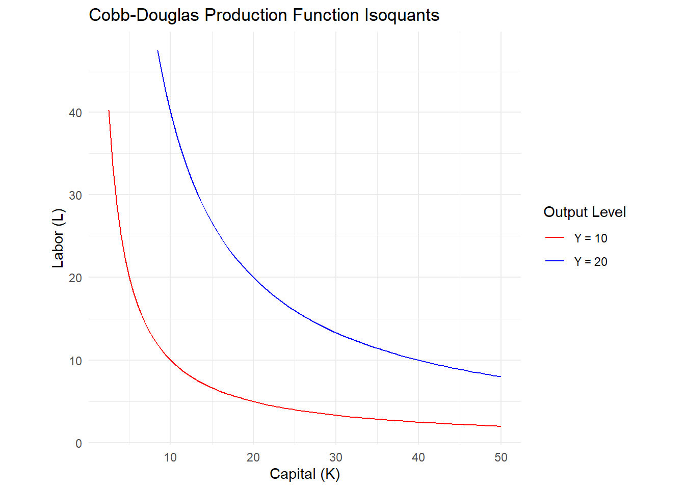
# Define the per-worker production function
f_k <- function(k) {
  k^0.5
}

# Generate a sequence of k values
k_values <- seq(0, 50, by = 0.1)

# Calculate y for each k
y_values <- f_k(k_values)

# Create a dataframe for plotting
data <- data.frame(k = k_values, y = y_values)

# Plot y as a function of k using ggplot
ggplot(data, aes(x = k, y = y)) +
  geom_line(color = "blue") +
  labs(title = "Per-worker Production Function: $y = k^0.5$",
       x = "Capital per worker (k)",
       y = "Output per worker (y)") +
  theme_minimal()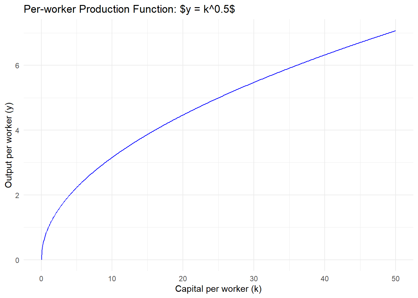
The change in capital is given by: $ K=s Y- d K $ where:
\(s\) is the saving rate.
\(d\) is the depreciation rate.
Key additional assumptions
The rest is basic algebra
Divide the capital accumulation equation by \(K\): $ = s - d $
\[ \frac{\Delta{K}}{K}=s \frac{Y}{K}-d=s \frac{\frac{Y}{L}}{\frac{K}{L}}-d=s \frac{y}{k}-d \]
Notice that: \[ \frac{\Delta{k}}{k}=\frac{\Delta{K}}{K}-\frac{\Delta{L}}{L}=\frac{\Delta{K}}{K}-n \Rightarrow \frac{\Delta{K}}{K}=\frac{\Delta{k}}{k}+n \]
We get:
\[ \frac{\Delta{k}}{k}+n=s \frac{y}{k}-d \Rightarrow \Delta{k}=s y-(d+n) k \]
Because, the Solow model is dynamic, it assumes that each country converges to its steady state, where capital stops growing, i.e. \(\Delta K = 0\).
\(0= \Delta {k^{\star}}=s A (k^{\star})^\alpha-(d+n) k\) \(\Rightarrow\)
The steady state capial per worker is: \[ k^*=\left(\frac{s A}{n+ d}\right)^{\frac{1}{1-\alpha}} \]
And the steady state output per worker is:
\[ y^*=\left(\frac{s A}{n+d}\right)^{\frac{\alpha}{1-\alpha}} \] - The steady state ouput per worker is increasing in the saving rate (\(s\)), and decreasing in the population growth rate (\(n\)) and the depreciation rate (\(d\)).
import numpy as np
import matplotlib.pyplot as plt

# Adjusted parameters for the Solow model
n = 0.03  # population growth rate
d = 0.06  # depreciation rate
s = 0.2   # saving rate
s_prime = 0.4  # new saving rate
alpha = 0.3  # capital's share of income, for a Cobb-Douglas production function
k_max = 10  # maximum capital to plot

# Define the production function, for simplicity we assume a Cobb-Douglas production function
def f(k):
    return k**alpha

# Create a grid of k (capital per worker) values
k = np.linspace(0.00, k_max, 200)  # Start from 0.01 to avoid division by zero

# Calculate output per worker
y = f(k)

# Calculate investment (saving) per worker
sy = s * y
sy_prime = s_prime * y

# Calculate break-even investment level (depreciation plus population growth)
ndk = (n + d) * k

# Plot the Solow model
plt.figure(figsize=(10, 6))

# Plot the production function y = f(k)
plt.plot(k, y, label='y = f(k)', color='black')

# Plot the saving function s * f(k)
plt.plot(k, sy, label='sy', color='blue')


# Plot the (n+d)k line
plt.plot(k, ndk, label='(n+d)k', linestyle='--', color='grey')

# Add annotations for the steady state levels of capital
k_star = (s / (n + d))**(1 / (1 - alpha))


plt.axvline(x=k_star, color='blue', linestyle=':', linewidth=1)


# Add labels and title
plt.xlabel('Capital per worker, k')
plt.ylabel('Output, investment, and depreciation per worker')
plt.title('An Increase in the Saving Rate in the Solow Model')

# Add a legend
plt.legend()

# Show the plot with a grid
plt.grid(True)
plt.show()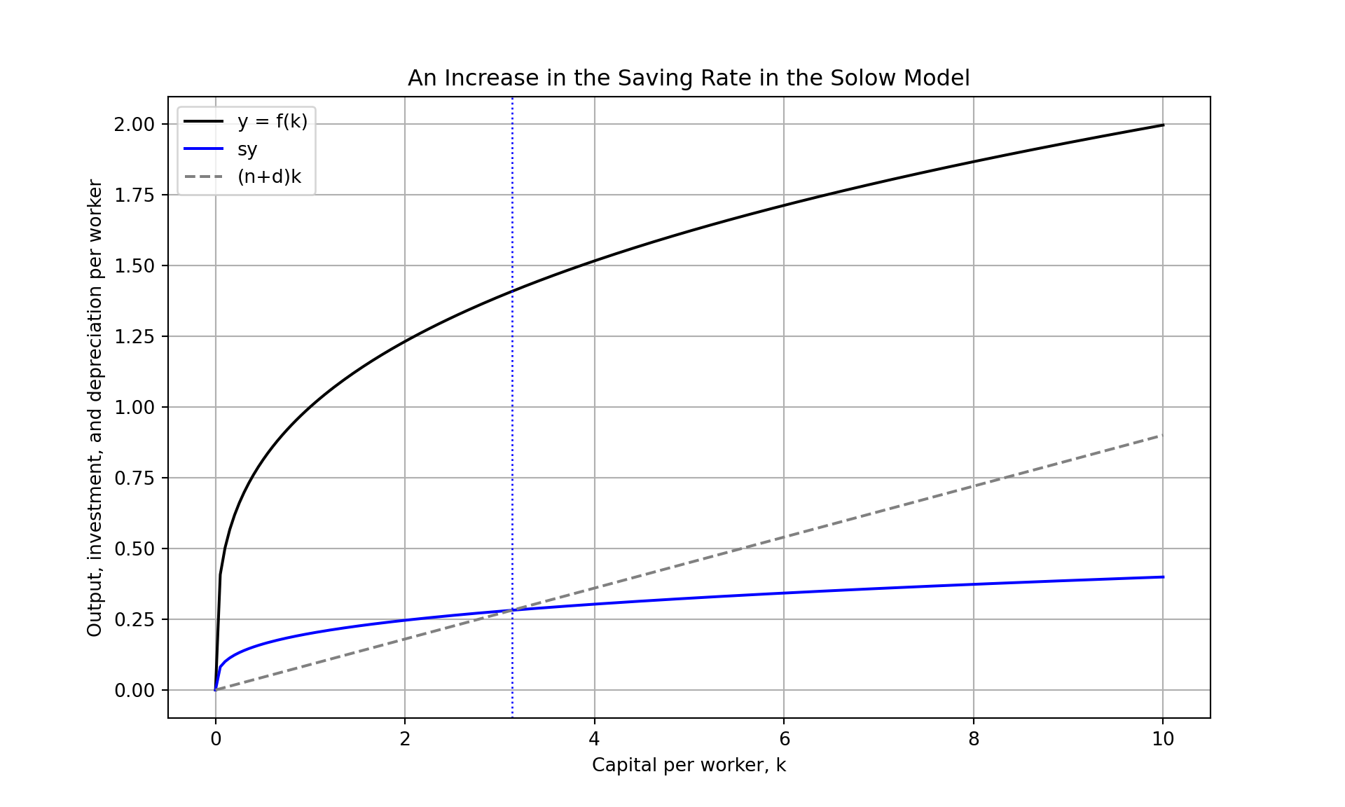
import numpy as np
import matplotlib.pyplot as plt

# Adjusted parameters for the Solow model
n = 0.03  # population growth rate
d = 0.06  # depreciation rate
s = 0.2   # saving rate
s_prime = 0.4  # new saving rate
alpha = 0.3  # capital's share of income, for a Cobb-Douglas production function
k_max = 10  # maximum capital to plot

# Define the production function, for simplicity we assume a Cobb-Douglas production function
def f(k):
    return k**alpha

# Create a grid of k (capital per worker) values
k = np.linspace(0.00, k_max, 200)  # Start from 0.01 to avoid division by zero

# Calculate output per worker
y = f(k)

# Calculate investment (saving) per worker
sy = s * y
sy_prime = s_prime * y

# Calculate break-even investment level (depreciation plus population growth)
ndk = (n + d) * k

# Plot the Solow model
plt.figure(figsize=(10, 6))

# Plot the production function y = f(k)
plt.plot(k, y, label='y = f(k)', color='black')

# Plot the saving function s * f(k)
plt.plot(k, sy, label='sy', color='blue')

# Plot the new saving function s' * f(k)
plt.plot(k, sy_prime, label="s'y", color='cyan')

# Plot the (n+d)k line
plt.plot(k, ndk, label='(n+d)k', linestyle='--', color='grey')

# Add annotations for the steady state levels of capital
k_star = (s / (n + d))**(1 / (1 - alpha))
k_star_prime = (s_prime / (n + d))**(1 / (1 - alpha))

plt.axvline(x=k_star, color='blue', linestyle=':', linewidth=1)
plt.axvline(x=k_star_prime, color='cyan', linestyle=':', linewidth=1)

# Add labels and title
plt.xlabel('Capital per worker, k')
plt.ylabel('Output, investment, and depreciation per worker')
plt.title('An Increase in the Saving Rate in the Solow Model')

# Add a legend
plt.legend()

# Show the plot with a grid
plt.grid(True)
plt.show()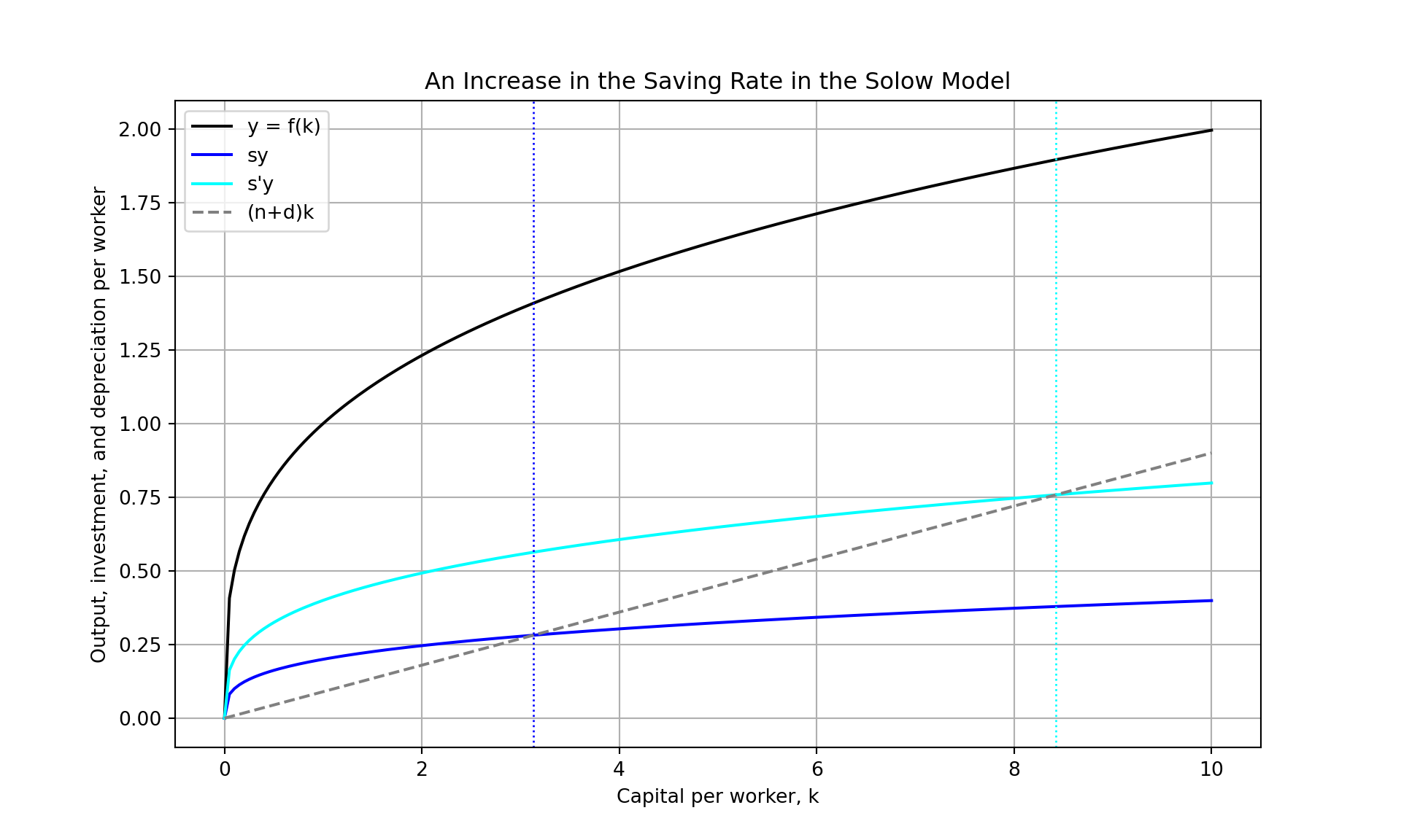
Why are some countries rich (have high per worker GDP) and others are poor (have low per worker GDP)?
Solow model: if all countries are in their steady states, then:
Rich countries have higher saving (investment) rates than poor countries
Rich countries have lower population growth rates than poor countries
\[ Y = A K^{\alpha}L^{(1-\alpha)} \] - Using the growth rate formulas, the growth of \(Y\) is:
\[ \frac{\Delta Y}{Y} = \frac{\Delta A}{A} + \alpha \frac{\Delta K}{K} + \left(1-\alpha \right)\frac{\Delta L}{L} \] - This is called a growth accounting equation
\[ \frac{\Delta A}{A} = \frac{\Delta Y}{Y} - \alpha \frac{\Delta K}{K} - \left(1-\alpha \right)\frac{\Delta L}{L} \]